An Introductory Example - Python Programming for Economics and Finance

3.1Overview¶

We’re now ready to start learning the Python language itself.

In this lecture, we will write and then pick apart small Python programs.

The objective is to introduce you to basic Python syntax and data structures.

Deeper concepts will be covered in later lectures.

You should have read the lecture on getting started with Python before beginning this one.

3.2The Task: Plotting a White Noise Process¶

Suppose we want to simulate and plot the white noise process $\epsilon_0, \epsilon_1, \ldots, \epsilon_T$ , where each draw $\epsilon_t$ is independent standard normal.

In other words, we want to generate figures that look something like this:

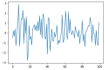
(Here $t$ is on the horizontal axis and $\epsilon_t$ is on the vertical axis.)

We’ll do this in several different ways, each time learning something more about Python.

3.3Version 1¶

Here are a few lines of code that perform the task we set

import numpy as np
import matplotlib.pyplot as plt

ϵ_values = np.random.randn(100)
plt.plot(ϵ_values)
plt.show()

Let’s break this program down and see how it works.

3.3.1Imports¶

The first two lines of the program import functionality from external code libraries.

The first line imports NumPy, a favorite Python package for tasks like

working with arrays (vectors and matrices)
common mathematical functions like cos and sqrt
generating random numbers
linear algebra, etc.

After import numpy as np we have access to these attributes via the syntax np.attribute.

Here’s two more examples

np.sqrt(4)

np.float64(2.0)

np.log(4)

np.float64(1.3862943611198906)

3.3.1.1Why So Many Imports?¶

Python programs typically require multiple import statements.

The reason is that the core language is deliberately kept small, so that it’s easy to learn, maintain and improve.

When you want to do something interesting with Python, you almost always need to import additional functionality.

3.3.1.2Packages¶

As stated above, NumPy is a Python package.

Packages are used by developers to organize code they wish to share.

In fact, a package is just a directory containing

files with Python code --- called modules in Python speak
possibly some compiled code that can be accessed by Python (e.g., functions compiled from C or FORTRAN code)
a file called __init__.py that specifies what will be executed when we type import package_name

You can check the location of your __init__.py for NumPy in python by running the code:

import numpy as np

print(np.__file__)

3.3.1.3Subpackages¶

Consider the line ϵ_values = np.random.randn(100).

Here np refers to the package NumPy, while random is a subpackage of NumPy.

Subpackages are just packages that are subdirectories of another package.

For instance, you can find folder random under the directory of NumPy.

3.3.2Importing Names Directly¶

Recall this code that we saw above

import numpy as np

np.sqrt(4)

np.float64(2.0)

Here’s another way to access NumPy’s square root function

from numpy import sqrt

sqrt(4)

np.float64(2.0)

This is also fine.

The advantage is less typing if we use sqrt often in our code.

The disadvantage is that, in a long program, these two lines might be separated by many other lines.

Then it’s harder for readers to know where sqrt came from, should they wish to.

3.3.3Random Draws¶

Returning to our program that plots white noise, the remaining three lines after the import statements are

ϵ_values = np.random.randn(100)
plt.plot(ϵ_values)
plt.show()

The first line generates 100 (quasi) independent standard normals and stores them in ϵ_values.

The next two lines genererate the plot.

We can and will look at various ways to configure and improve this plot below.

3.4Alternative Implementations¶

Let’s try writing some alternative versions of our first program, which plotted IID draws from the standard normal distribution.

The programs below are less efficient than the original one, and hence somewhat artificial.

But they do help us illustrate some important Python syntax and semantics in a familiar setting.

3.4.1A Version with a For Loop¶

Here’s a version that illustrates for loops and Python lists.

ts_length = 100
ϵ_values = []   # empty list

for i in range(ts_length):
    e = np.random.randn()
    ϵ_values.append(e)

plt.plot(ϵ_values)
plt.show()

In brief,

The first line sets the desired length of the time series.
The next line creates an empty list called ϵ_values that will store the $\epsilon_t$ values as we generate them.
The statement # empty list is a comment, and is ignored by Python’s interpreter.
The next three lines are the for loop, which repeatedly draws a new random number $\epsilon_t$ and appends it to the end of the list ϵ_values.
The last two lines generate the plot and display it to the user.

Let’s study some parts of this program in more detail.

3.4.2Lists¶

Consider the statement ϵ_values = [], which creates an empty list.

Lists are a native Python data structure used to group a collection of objects.

Items in lists are ordered, and duplicates are allowed in lists.

For example, try

x = [10, 'foo', False]
type(x)

list

The first element of x is an integer, the next is a string, and the third is a Boolean value.

When adding a value to a list, we can use the syntax list_name.append(some_value)

[10, 'foo', False]

x.append(2.5)
x

[10, 'foo', False, 2.5]

Here append() is what’s called a method, which is a function “attached to” an object---in this case, the list x.

We’ll learn all about methods later on, but just to give you some idea,

Python objects such as lists, strings, etc. all have methods that are used to manipulate data contained in the object.
String objects have string methods, list objects have list methods, etc.

Another useful list method is pop()

[10, 'foo', False, 2.5]

x.pop()

2.5

[10, 'foo', False]

Lists in Python are zero-based (as in C, Java or Go), so the first element is referenced by x[0]

x[0]   # first element of x

10

x[1]   # second element of x

'foo'

3.4.3The For Loop¶

Now let’s consider the for loop from the program above, which was

for i in range(ts_length):
    e = np.random.randn()
    ϵ_values.append(e)

Python executes the two indented lines ts_length times before moving on.

These two lines are called a code block, since they comprise the “block” of code that we are looping over.

Unlike most other languages, Python knows the extent of the code block only from indentation.

In our program, indentation decreases after line ϵ_values.append(e), telling Python that this line marks the lower limit of the code block.

More on indentation below---for now, let’s look at another example of a for loop

animals = ['dog', 'cat', 'bird']
for animal in animals:
    print("The plural of " + animal + " is " + animal + "s")

The plural of dog is dogs
The plural of cat is cats
The plural of bird is birds

This example helps to clarify how the for loop works: When we execute a loop of the form

for variable_name in sequence:
    <code block>

The Python interpreter performs the following:

For each element of the sequence, it “binds” the name variable_name to that element and then executes the code block.

3.4.4A Comment on Indentation¶

In discussing the for loop, we explained that the code blocks being looped over are delimited by indentation.

In fact, in Python, all code blocks (i.e., those occurring inside loops, if clauses, function definitions, etc.) are delimited by indentation.

Thus, unlike most other languages, whitespace in Python code affects the output of the program.

Once you get used to it, this is a good thing: It

forces clean, consistent indentation, improving readability
removes clutter, such as the brackets or end statements used in other languages

On the other hand, it takes a bit of care to get right, so please remember:

The line before the start of a code block always ends in a colon
- for i in range(10):
- if x > y:
- while x < 100:
- etc.
All lines in a code block must have the same amount of indentation.
The Python standard is 4 spaces, and that’s what you should use.

3.4.5While Loops¶

The for loop is the most common technique for iteration in Python.

But, for the purpose of illustration, let’s modify the program above to use a while loop instead.

ts_length = 100
ϵ_values = []
i = 0
while i < ts_length:
    e = np.random.randn()
    ϵ_values.append(e)
    i = i + 1
plt.plot(ϵ_values)
plt.show()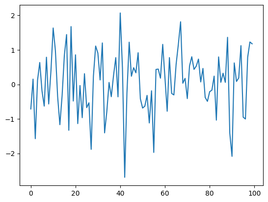

A while loop will keep executing the code block delimited by indentation until the condition (i < ts_length) is satisfied.

In this case, the program will keep adding values to the list ϵ_values until i equals ts_length:

i == ts_length #the ending condition for the while loop

True

Note that

the code block for the while loop is again delimited only by indentation.
the statement i = i + 1 can be replaced by i += 1.

3.5Another Application¶

Let’s do one more application before we turn to exercises.

In this application, we plot the balance of a bank account over time.

There are no withdraws over the time period, the last date of which is denoted by $T$ .

The initial balance is $b_0$ and the interest rate is $r$ .

The balance updates from period $t$ to $t+1$ according to $b_{t+1} = (1 + r) b_t$ .

In the code below, we generate and plot the sequence $b_0, b_1, \ldots, b_T$ .

Instead of using a Python list to store this sequence, we will use a NumPy array.

r = 0.025         # interest rate
T = 50            # end date
b = np.empty(T+1) # an empty NumPy array, to store all b_t
b[0] = 10         # initial balance

for t in range(T):
    b[t+1] = (1 + r) * b[t]

plt.plot(b, label='bank balance')
plt.legend()
plt.show()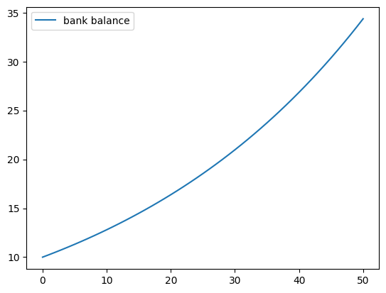

The statement b = np.empty(T+1) allocates storage in memory for T+1 (floating point) numbers.

These numbers are filled in by the for loop.

Allocating memory at the start is more efficient than using a Python list and append, since the latter must repeatedly ask for storage space from the operating system.

Notice that we added a legend to the plot --- a feature you will be asked to use in the exercises.

3.6Exercises¶

Now we turn to exercises. It is important that you complete them before continuing, since they present new concepts we will need.

Exercise 1

Your first task is to simulate and plot the correlated time series

x_{t+1} = \alpha \, x_t + \epsilon_{t+1} \quad \text{where} \quad x_0 = 0 \quad \text{and} \quad t = 0,\ldots,T

(1)

The sequence of shocks $\{\epsilon_t\}$ is assumed to be IID and standard normal.

In your solution, restrict your import statements to

import numpy as np
import matplotlib.pyplot as plt

Set $T=200$ and $\alpha = 0.9$ .

Solution to Exercise 1

Here’s one solution.

α = 0.9
T = 200
x = np.empty(T+1)
x[0] = 0

for t in range(T):
    x[t+1] = α * x[t] + np.random.randn()

plt.plot(x)
plt.show()

Solution to Exercise 2

α_values = [0.0, 0.8, 0.98]
T = 200
x = np.empty(T+1)

for α in α_values:
    x[0] = 0
    for t in range(T):
        x[t+1] = α * x[t] + np.random.randn()
    plt.plot(x, label=f'$\\alpha = {α}$')

plt.legend()
plt.show()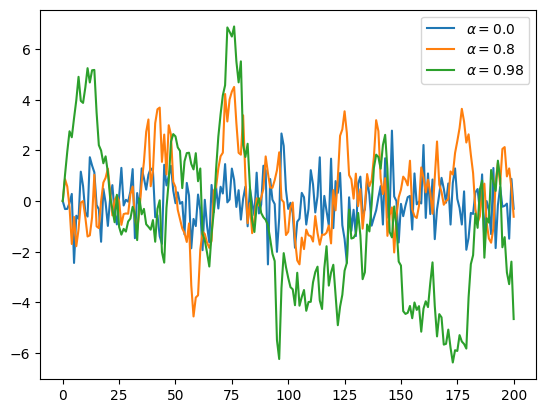

Solution to Exercise 3

Here’s one solution:

α = 0.9
T = 200
x = np.empty(T+1)
x[0] = 0

for t in range(T):
    x[t+1] = α * np.abs(x[t]) + np.random.randn()

plt.plot(x)
plt.show()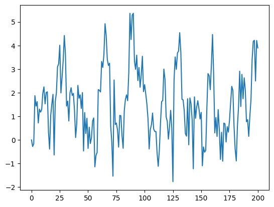

Exercise 4

One important aspect of essentially all programming languages is branching and conditions.

In Python, conditions are usually implemented with if--else syntax.

Here’s an example, that prints -1 for each negative number in an array and 1 for each nonnegative number

numbers = [-9, 2.3, -11, 0]

for x in numbers:
    if x < 0:
        print(-1)
    else:
        print(1)

-1
1
-1
1

Now, write a new solution to Exercise 3 that does not use an existing function to compute the absolute value.

Replace this existing function with an if--else condition.

Solution to Exercise 4

Here’s one way:

α = 0.9
T = 200
x = np.empty(T+1)
x[0] = 0

for t in range(T):
    if x[t] < 0:
        abs_x = - x[t]
    else:
        abs_x = x[t]
    x[t+1] = α * abs_x + np.random.randn()

plt.plot(x)
plt.show()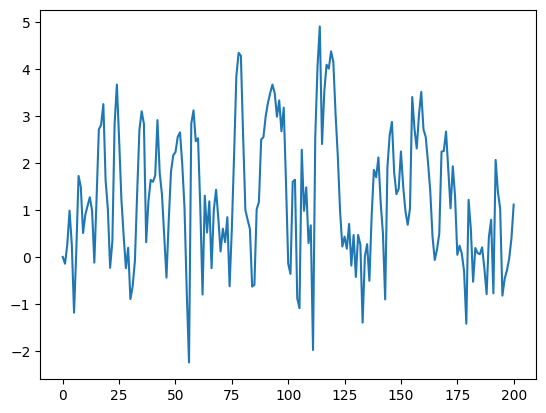

Here’s a shorter way to write the same thing:

α = 0.9
T = 200
x = np.empty(T+1)
x[0] = 0

for t in range(T):
    abs_x = - x[t] if x[t] < 0 else x[t]
    x[t+1] = α * abs_x + np.random.randn()

plt.plot(x)
plt.show()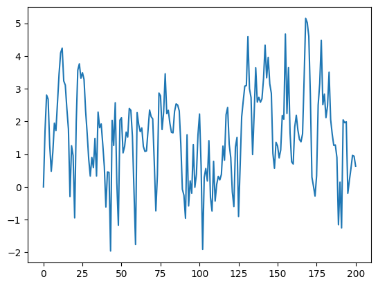

Exercise 5

Here’s a harder exercise, that takes some thought and planning.

The task is to compute an approximation to π using Monte Carlo.

Use no imports besides

import numpy as np

Solution to Exercise 5

Consider the circle of diameter 1 embedded in the unit square.

Let $A$ be its area and let $r=1/2$ be its radius.

If we know π then we can compute $A$ via $A = \pi r^2$ .

But here the point is to compute π, which we can do by $\pi = A / r^2$ .

Summary: If we can estimate the area of a circle with diameter 1, then dividing by $r^2 = (1/2)^2 = 1/4$ gives an estimate of π.

We estimate the area by sampling bivariate uniforms and looking at the fraction that falls into the circle.

n = 1000000 # sample size for Monte Carlo simulation

count = 0
for i in range(n):

    # drawing random positions on the square
    u, v = np.random.uniform(), np.random.uniform()

    # check whether the point falls within the boundary
    # of the unit circle centred at (0.5,0.5)
    d = np.sqrt((u - 0.5)**2 + (v - 0.5)**2)

    # if it falls within the inscribed circle, 
    # add it to the count
    if d < 0.5:
        count += 1

area_estimate = count / n

print(area_estimate * 4)  # dividing by radius**2

3.141716

3. An Introductory Example

3.1Overview¶

3.2The Task: Plotting a White Noise Process¶

3.3Version 1¶

3.3.1Imports¶

3.3.1.1Why So Many Imports?¶

3.3.1.2Packages¶

3.3.1.3Subpackages¶

3.3.2Importing Names Directly¶

3.3.3Random Draws¶

3.4Alternative Implementations¶

3.4.1A Version with a For Loop¶

3.4.2Lists¶

3.4.3The For Loop¶

3.4.4A Comment on Indentation¶

3.4.5While Loops¶

3.5Another Application¶

3.6Exercises¶